introduction

faer is a linear algebra library developed in the rust programming language. it exposes a high level abstraction over a lower level api, similar to the one offered by blas/lapack libraries, modified to better match the capabilities of modern computers, and allows tweaking the inner parameters of the various algorithms.

community

most of the discussion around the library happens on the discord server. users who have questions about using the library, performance issues, bug reports, etc, as well as people looking to contribute, are welcome to join the server!

bug reports and pull requests can also be posted on the github repository.

available features

• matrix creation and basic operation (addition, subtraction, multiplication, etc.),
• high performance matrix multiplication,
• triangular solvers,
• cholesky decomposition, llt, ldlt, and bunch-kaufman lblt,
• lu decomposition, with partial or full pivoting,
• qr decomposition, with or without column pivoting.
• svd decomposition.
• eigenvalue decomposition for hermitian and non hermitian (real or complex) matrices.
• sparse algorithms.

future plans

• n-dimensional tensor structures and operations.
• gpu acceleration.

to use faer in your project, you can add the required dependency to your cargo.toml file.

[dependencies]
faer = "0.19"

for day-to-day development, we recommend enabling optimizations for faer, since the layers of generics can add considerable overhead in unoptimized builds. this can be done by adding the following to Cargo.toml

[profile.dev.package.faer]
opt-level = 3

we recommend new users to skim the user guide provided in the sidebar, and defer to the docs for more detailed information.

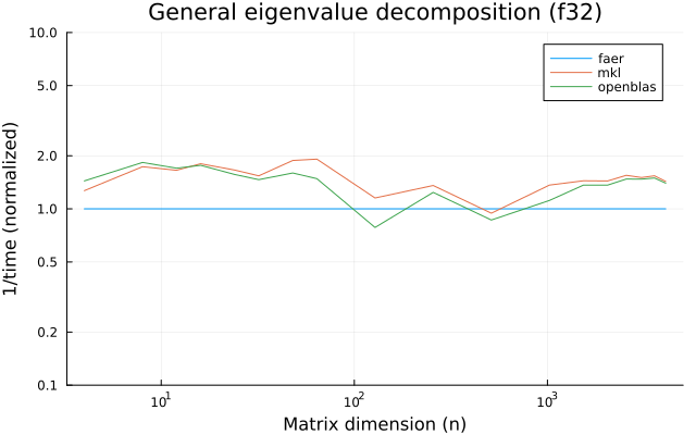
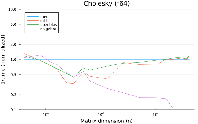
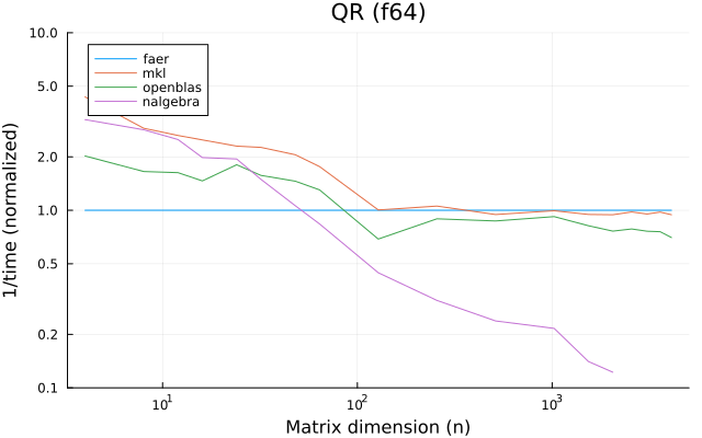
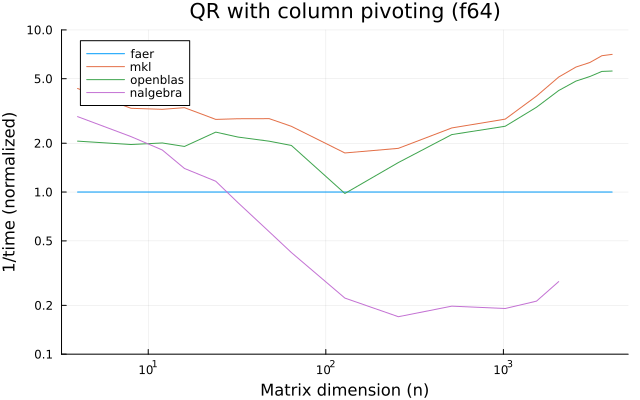
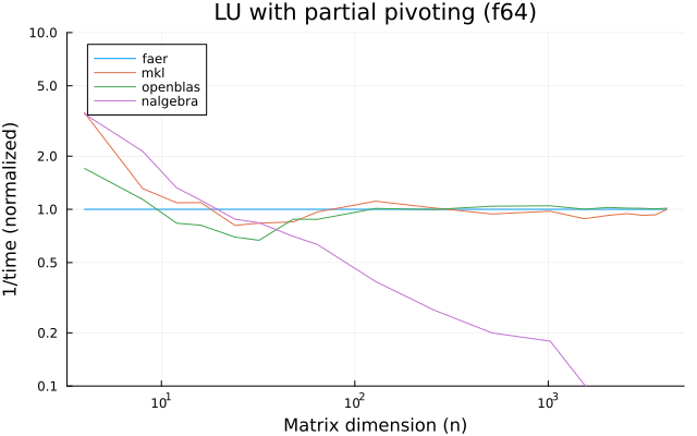
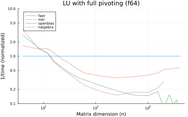
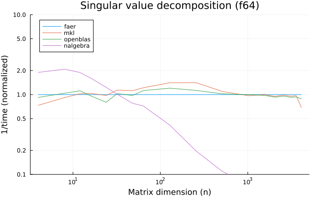
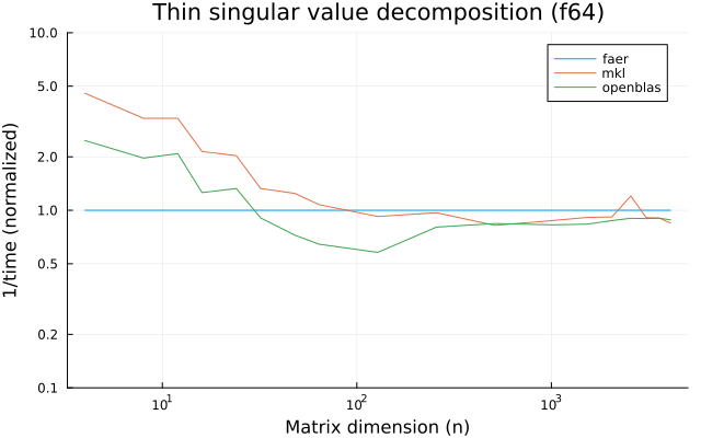
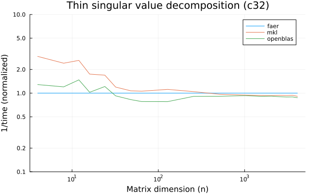
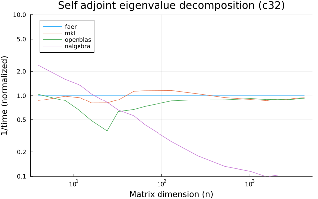
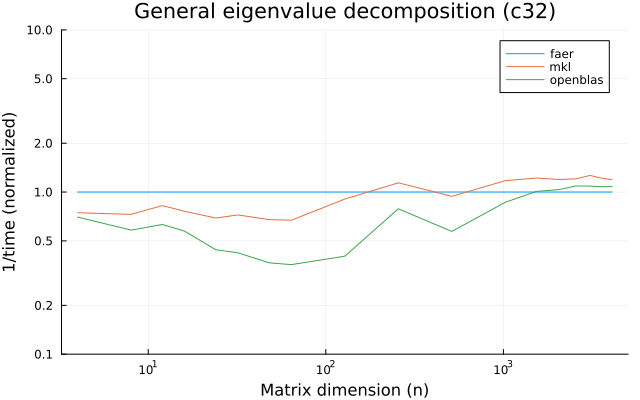
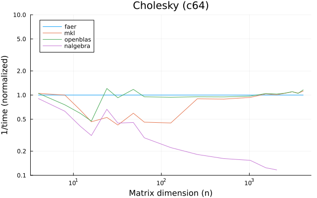
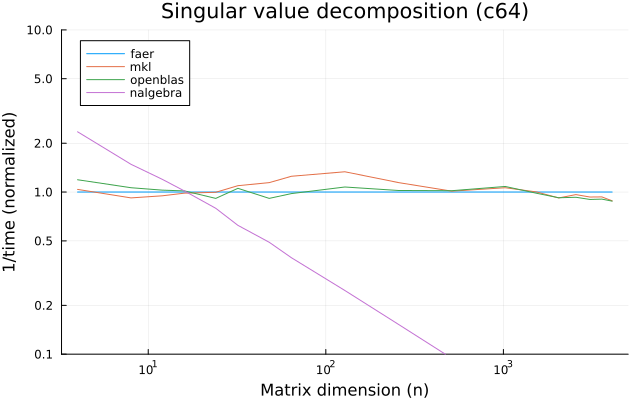
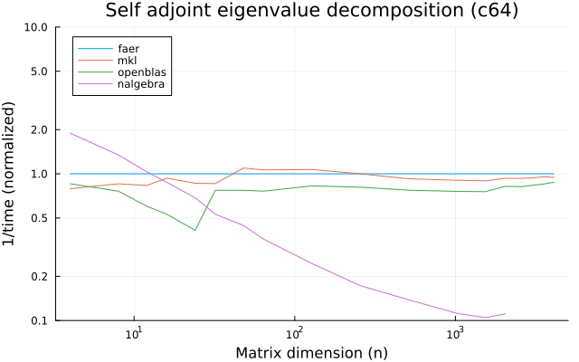
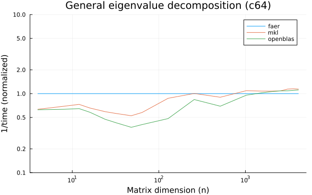
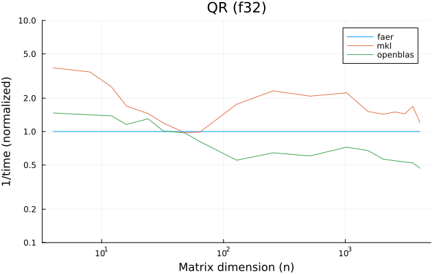
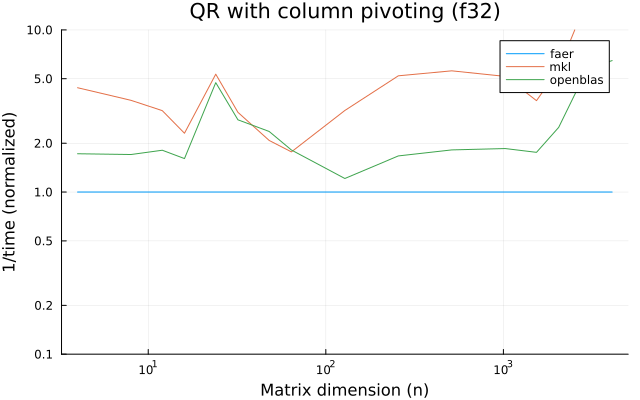
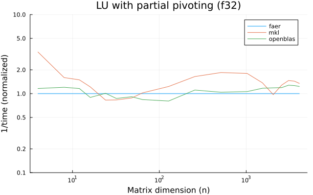
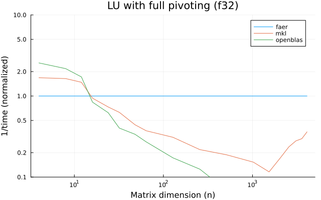
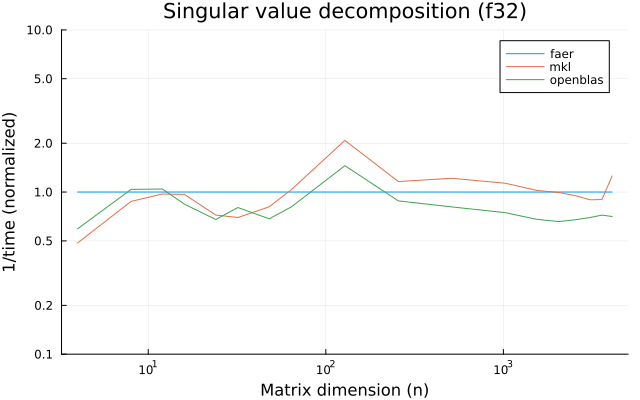
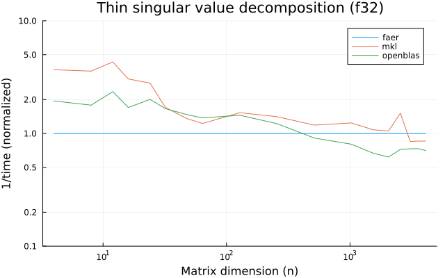
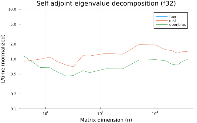
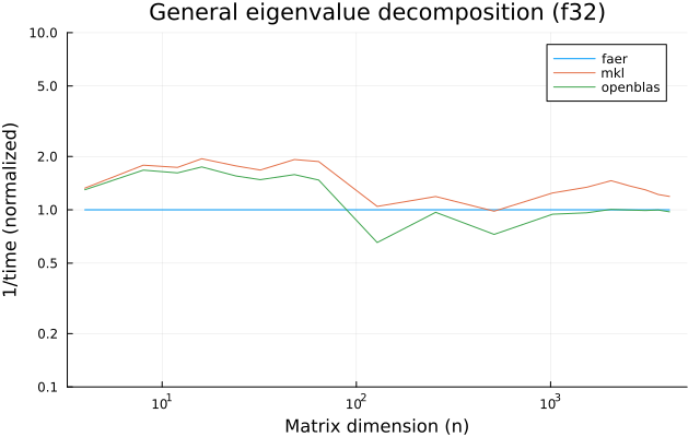
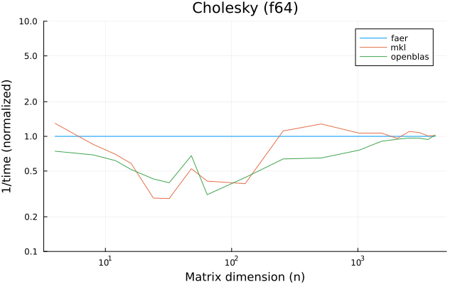
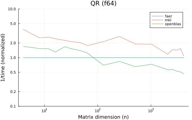
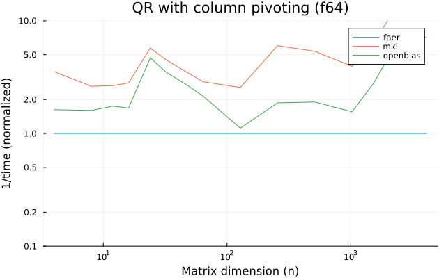
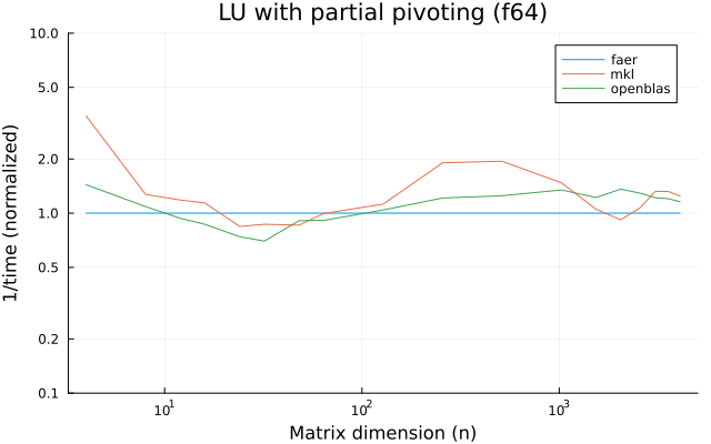
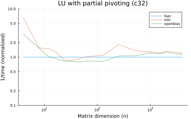
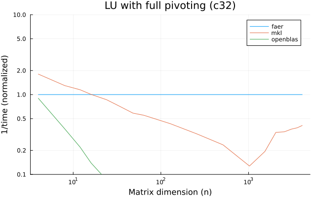
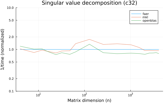
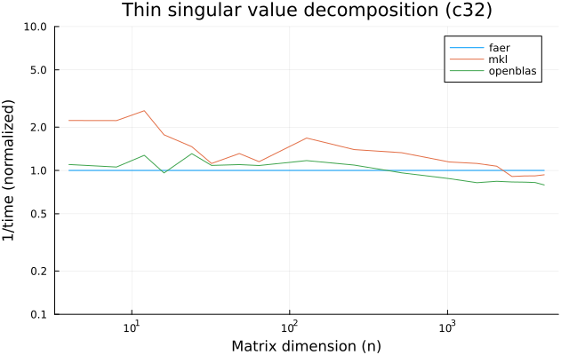
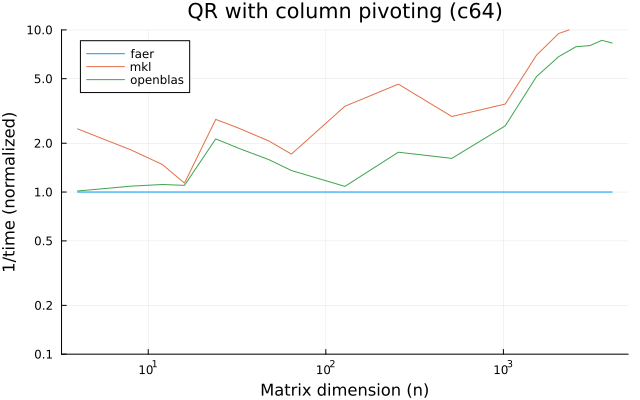
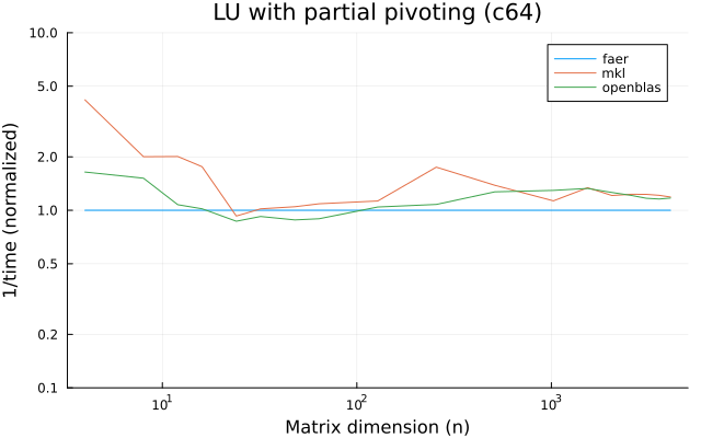
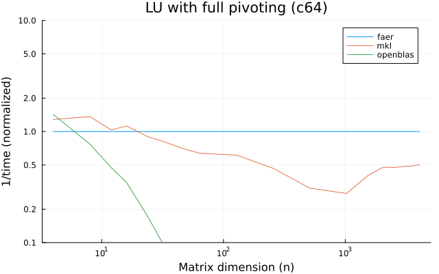
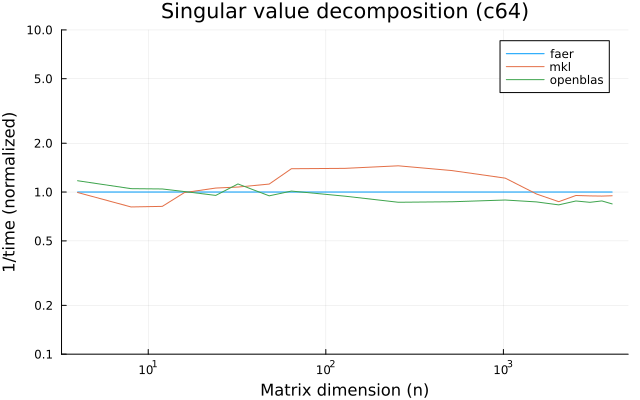
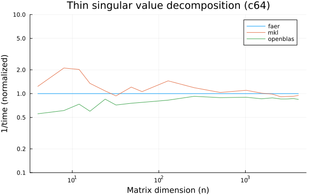
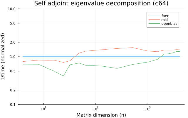
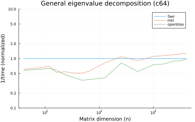
the benchmarks were run on an 11th gen intel(r) core(tm) i5-11400 @ 2.60ghz with 1 thread (hyperthreading off).

all computations are done on column major matrices.

the plots are normalized so that the faer line is set to 1.0.

higher is better on all the plots.

last updated: 2024-05-25

f32

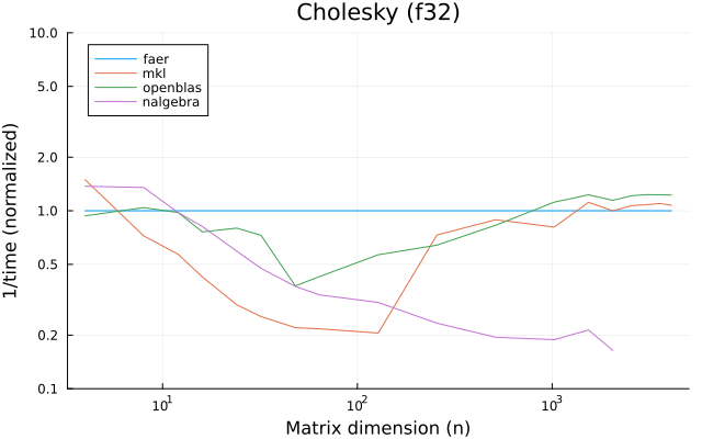
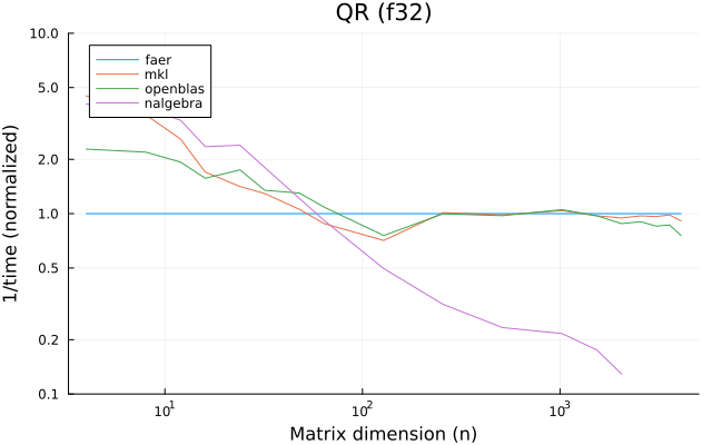
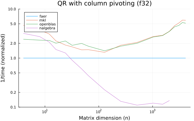
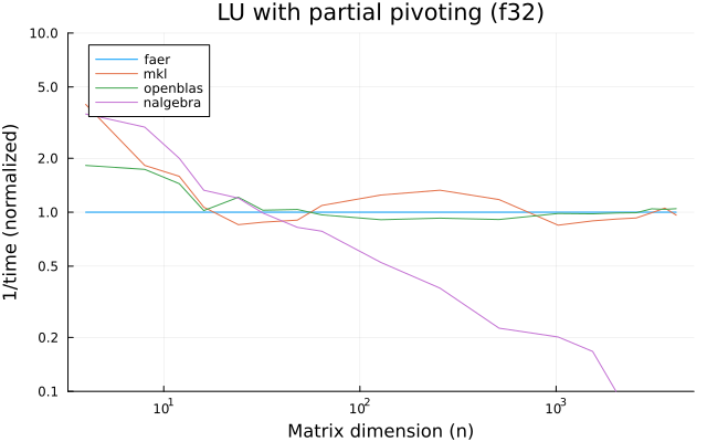
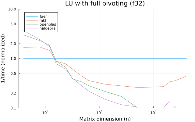
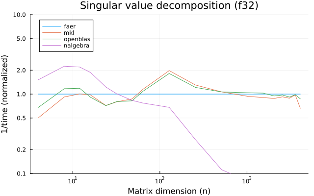
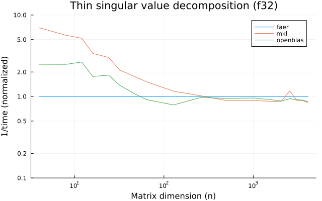
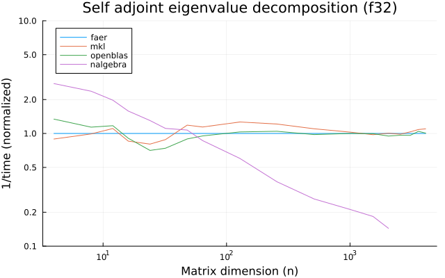
f64

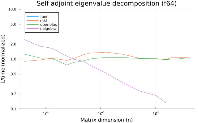
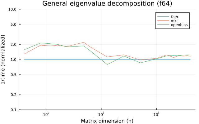
c32

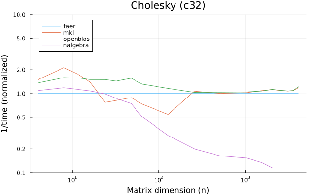
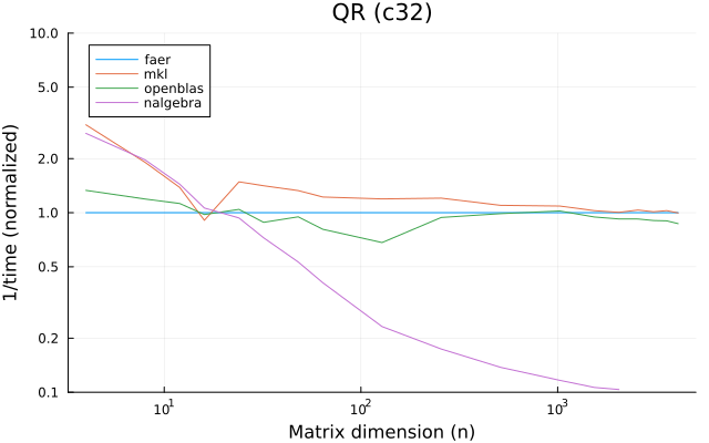
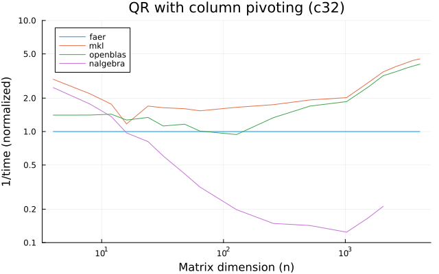
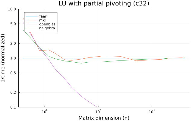
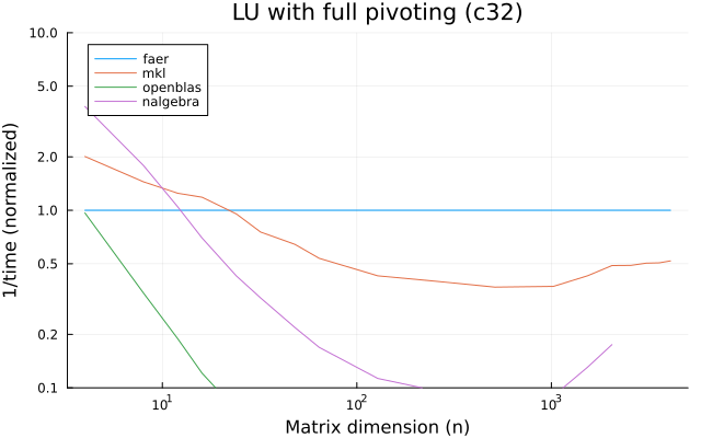
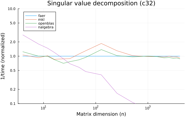
c64

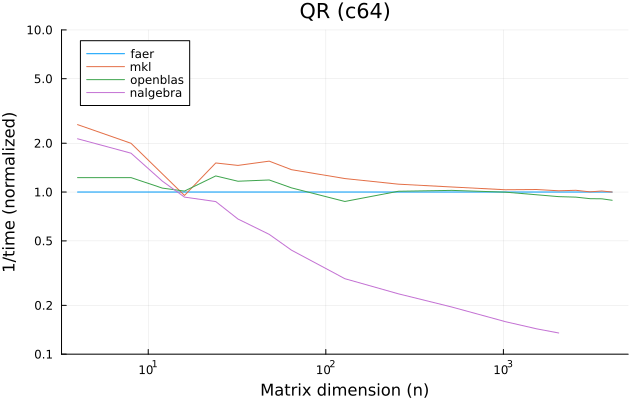
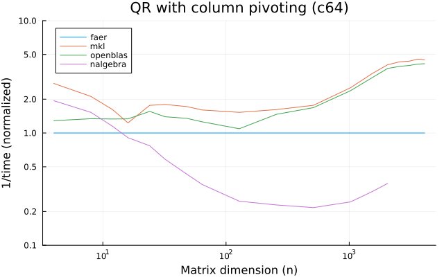
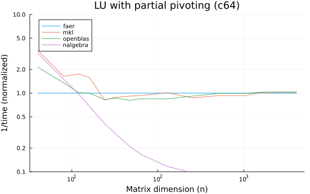
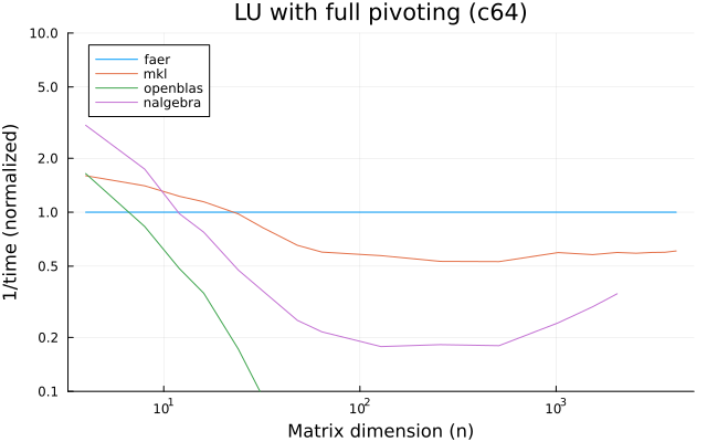
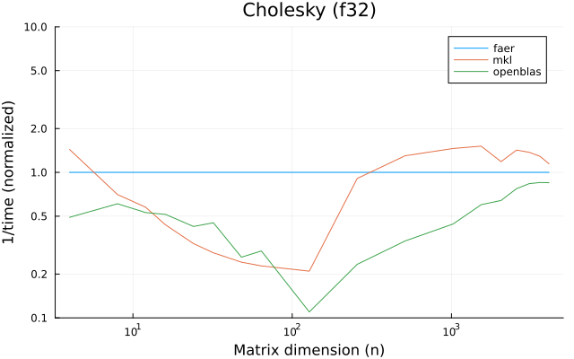
the benchmarks were run on an 11th gen intel(r) core(tm) i5-11400 @ 2.60ghz with 6 threads (hyperthreading off).

all computations are done on column major matrices.

the plots are normalized so that the faer line is set to 1.0.

higher is better on all the plots.

last updated: 2024-05-25

f32

f64

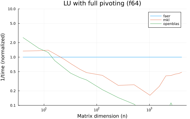
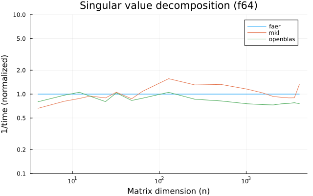
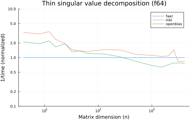
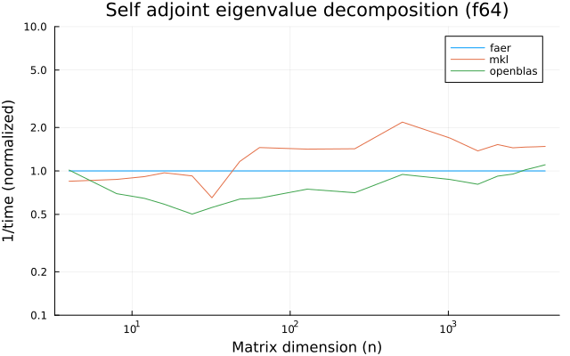
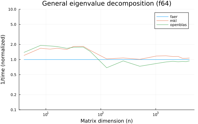
c32

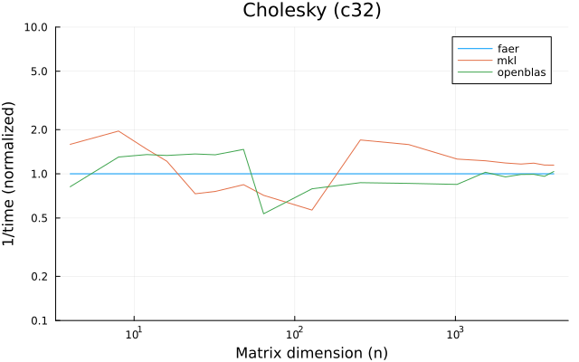
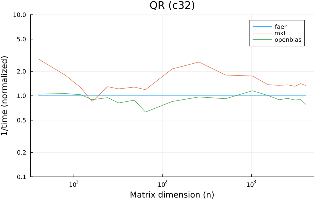
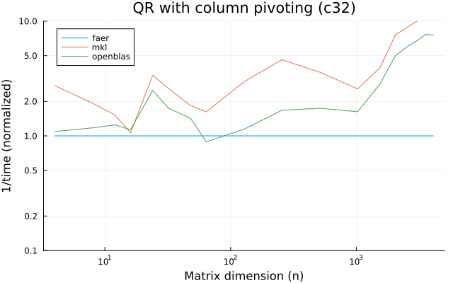
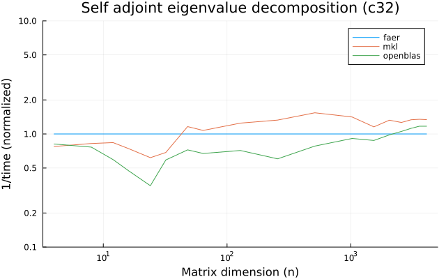
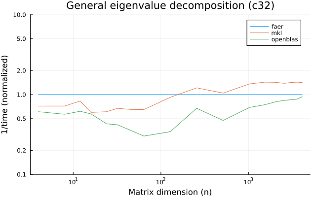
c64

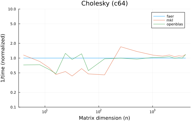
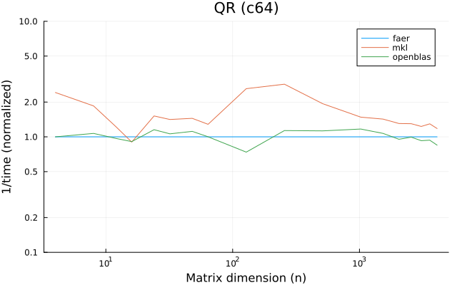
Matrix management

Creating a matrix

faer provides several ways to create dense matrices and matrix views.

The main matrix types are Mat, MatRef and MatMut, which can be thought of as being analogous to Vec, &[_] and &mut [_].

• Mat owns its data, provides read-write access to it, and can be resized after creation.
• MatRef provides read-only access to the underlying data.
• MatMut provides read-write access to the underlying data.

The most flexible way to initialize a matrix is to initialize a zero matrix, then fill out the values by hand.

use faer::Mat;

let mut a = Mat::<f64>::zeros(4, 3);

for j in 0..a.ncols() {
    for i in 0..a.nrows() {
        a[(i, j)] = 9.0;
    }
}

Given a callable object that outputs the matrix elements, Mat::from_fn, can also be used.

use faer::Mat;

let a = Mat::from_fn(3, 4, |i, j| (i + j) as f64);

For common matrices such as the zero matrix and the identity matrix, shorthands are provided.

use faer::Mat;

// creates a 10×4 matrix whose values are all `0.0`.
let a = Mat::<f64>::zeros(10, 4);

// creates a 5×4 matrix containing `0.0` except on the main diagonal,
// which contains `1.0` instead.
let a = Mat::<f64>::identity(5, 4);

In some cases, users may wish to avoid the cost of initializing the matrix to zero, in which case, unsafe code may be used to allocate an uninitialized matrix, which can then be filled out before it's used.

// `a` is initially a 0×0 matrix.
let mut a = Mat::<f64>::with_capacity(4, 3);

// `a` is now a 4×3 matrix, whose values are uninitialized.
unsafe { a.set_dims(4, 3) };

for j in 0..a.ncols() {
    for i in 0..a.nrows() {
        // we cannot write `a[(i, j)] = 9.0`, as that would
        // create a reference to uninitialized data,
        // which is currently disallowed by Rust.
        a.write(i, j, 9.0);

        // we can also skip the bound checks using
        // read_unchecked and write_unchecked
        unsafe { a.write_unchecked(i, j, 9.0) };
    }
}

Creating a matrix view

In some situations, it may be desirable to create a matrix view over existing data. In that case, we can use MatRef (or MatMut for mutable views).

They can be created in a safe way using:

• mat::from_column_major_slice,
• mat::from_row_major_slice,
• mat::from_column_major_slice_mut,
• mat::from_row_major_slice_mut,

for contiguous matrix storage, or:

• mat::from_column_major_slice_with_stride,
• mat::from_row_major_slice_with_stride,
• mat::from_column_major_slice_with_stride_mut,
• mat::from_row_major_slice_with_stride_mut,

for strided matrix storage.

An unsafe lower level pointer API is also provided for handling uninitialized data or arbitrary strides using mat::from_raw_parts and mat::from_raw_parts_mut.

Converting to a view

A Mat instance m can be converted to MatRef or MatMut by writing m.as_ref() or m.as_mut().

Reborrowing a mutable view

Immutable matrix views can be freely copied around, since they are non-owning wrappers around a pointer and the matrix dimensions/strides.

Mutable matrices however are limited by Rust's borrow checker. Copying them would be unsound since only a single active mutable view is allowed at a time.

This means the following code does not compile.

use faer::{Mat, MatMut};

fn takes_view_mut(m: MatMut<f64>) {}

let mut a = Mat::<f64>::new();
let view = a.as_mut();

takes_view_mut(view);

// This would have failed to compile since `MatMut` is never `Copy`
// takes_view_mut(view);

The alternative is to temporarily give up ownership over the data, by creating a view with a shorter lifetime, then recovering the ownership when the view is no longer being used.

This is also called reborrowing.

use faer::{Mat, MatMut, MatRef};
use reborrow::*;

fn takes_view(m: MatRef<f64>) {}
fn takes_view_mut(m: MatMut<f64>) {}

let mut a = Mat::<f64>::new();
let mut view = a.as_mut();

takes_view_mut(view.rb_mut());
takes_view_mut(view.rb_mut());
takes_view(view.rb()); // We can also reborrow immutably

{
    let short_view = view.rb_mut();

    // This would have failed to compile since we can't use the original view
    // while the reborrowed view is still being actively used
    // takes_view_mut(view);

    takes_view_mut(short_view);
}

// We can once again use the original view
takes_view_mut(view.rb_mut());

// Or consume it to convert it to an immutable view
takes_view(view.into_const());

Splitting a matrix view, slicing a submatrix

A matrix view can be split up along its row axis, column axis or both. This is done using MatRef::split_at_row, MatRef::split_at_col or MatRef::split_at (or MatMut::split_at_row_mut, MatMut::split_at_col_mut or MatMut::split_at_mut).

These functions take the middle index at which the split is performed, and return the two sides (in top/bottom or left/right order) or the four corners (top left, top right, bottom left, bottom right)

We can also take a submatrix using MatRef::subrows, MatRef::subcols or MatRef::submatrix (or MatMut::subrows_mut, MatMut::subcols_mut or MatMut::submatrix_mut).

Alternatively, we can also use MatRef::get or MatMut::get_mut, which take as parameters the row and column ranges.

⚠️Warning⚠️

Note that MatRef::submatrix (and MatRef::subrows, MatRef::subcols) takes as a parameter, the first row and column of the submatrix, then the number of rows and columns of the submatrix.

On the other hand, MatRef::get takes a range from the first row and column to the last row and column.

Matrix arithmetic operations

faer matrices implement most of the arithmetic operators, so two matrices can be added simply by writing &a + &b, the result of the expression is a faer::Mat, which allows simple chaining of operations (e.g. (&a + faer::scale(3.0) * &b) * &c), although at the cost of allocating temporary matrices.

temporary allocations can be avoided by using the zipped! api:

use faer::{Mat, zipped, unzipped};

let a = Mat::<f64>::zeros(4, 3);
let b = Mat::<f64>::zeros(4, 3);
let mut c = Mat::<f64>::zeros(4, 3);

// Sums `a` and `b` and stores the result in `c`.
zipped!(&mut c, &a, &b).for_each(|unzipped!(c, a, b)| *c = *a + *b);

// Sums `a`, `b` and `c` into a new matrix `d`.
let d = zipped!(&mut c, &a, &b).map(|unzipped!(c, a, b)| *a + *b + *c);

for matrix multiplication, the non-allocating api in-place is provided in the faer::linalg::matmul module.

use faer::{Mat, Parallelism};
use faer::linalg::matmul::matmul;

let a = Mat::<f64>::zeros(4, 3);
let b = Mat::<f64>::zeros(3, 5);

let mut c = Mat::<f64>::zeros(4, 5);

// Computes `faer::scale(3.0) * &a * &b` and stores the result in `c`.
matmul(c.as_mut(), a.as_ref(), b.as_ref(), None, 3.0, Parallelism::None);

// Computes `faer::scale(3.0) * &a * &b + 5.0 * &c` and stores the result in `c`.
matmul(c.as_mut(), a.as_ref(), b.as_ref(), Some(5.0), 3.0, Parallelism::None);

Solving a Linear System

several applications require solving a linear system of the form \(A x = b\). the recommended method can vary depending on the properties of \(A\), and the desired numerical accuracy.

\(A\) is triangular

in this case, one can use \(A\) and \(b\) directly to find \(x\), using the functions provided in faer::linalg::triangular_solve.

use faer::{Mat, Parallelism};
use faer::linalg::triangular_solve::solve_lower_triangular_in_place;

let a = Mat::<f64>::from_fn(4, 4, |i, j| if i >= j { 1.0 } else { 0.0 });
let b = Mat::<f64>::from_fn(4, 2, |i, j| (i - j) as f64);

let mut x = Mat::<f64>::zeros(4, 2);
x.copy_from(&b);
solve_lower_triangular_in_place(a.as_ref(), x.as_mut(), Parallelism::None);

// x now contains the approximate solution

in the case where \(A\) has a unit diagonal, one can use solve_unit_lower_triangular_in_place, which avoids reading the diagonal, and instead implicitly uses the value 1.0 as a replacement.

\(A\) is real-symmetric/complex-Hermitian

if \(A\) is Hermitian and positive definite, users can use the cholesky llt decomposition.

use faer::{mat, Side};
use faer::prelude::*;

let a = mat![
    [10.0, 2.0],
    [2.0, 10.0f64],
];
let b = mat![[15.0], [-3.0f64]];

// Compute the Cholesky decomposition,
// reading only the lower triangular half of the matrix.
let llt = a.cholesky(Side::Lower).unwrap();

let x = llt.solve(&b);

Low level API

alternatively, a lower-level api could be used to avoid temporary allocations. the corresponding code for other decompositions follows the same pattern, so we will skip similar examples for the remainder of this page.

use faer::{mat, Parallelism, Conj};
use faer::linalg::cholesky::llt::compute::cholesky_in_place_req;
use faer::linalg::cholesky::llt::compute::{cholesky_in_place, LltRegularization, LltParams};
use faer::linalg::cholesky::llt::solve::solve_in_place_req;
use faer::linalg::cholesky::llt::solve::solve_in_place_with_conj;
use dyn_stack::{PodStack, GlobalPodBuffer};

let a = mat![
    [10.0, 2.0],
    [2.0, 10.0f64],
];
let mut b = mat![[15.0], [-3.0f64]];

let mut llt = Mat::<f64>::zeros(2, 2);
let no_par = Parallelism::None;

// Compute the size and alignment of the required scratch space
let cholesky_memory = cholesky_in_place_req::<f64>(
    a.nrows(),
    Parallelism::None,
    LltParams::default(),
).unwrap();
let solve_memory = solve_in_place_req::<f64>(
    a.nrows(),
    b.ncols(),
    Parallelism::None,
).unwrap();

// Allocate the scratch space
let mut memory = GlobalPodBuffer::new(cholesky_memory.or(solve_memory));
let mut stack = PodStack::new(&mut mem);

// Compute the decomposition
llt.copy_from(&a);
cholesky_in_place(
    llt.as_mut(),
    LltRegularization::default(), // no regularization
    no_par,
    stack.rb_mut(),               // scratch space
    LltParams::default(),         // default settings
);
// Solve the linear system
solve_in_place_with_conj(llt.as_ref(), Conj::No, b.as_mut(), no_par, stack);

If \(A\) is not positive definite, the Bunch-Kaufman LBLT decomposition is recommended instead.

use faer::{mat, Side};
use faer::prelude::*;

let a = mat![
    [10.0, 2.0],
    [2.0, -10.0f64],
];
let b = mat![[15.0], [-3.0f64]];

// Compute the Bunch-Kaufman LBLT decomposition,
// reading only the lower triangular half of the matrix.
let lblt = a.lblt(Side::Lower);

let x = lblt.solve(&b);

\(A\) is square

for a square matrix \(A\), we can use the lu decomposition with partial pivoting, or the full pivoting variant which is slower but can be more accurate when the matrix is nearly singular.

use faer::mat;
use faer::prelude::*;

let a = mat![
    [10.0, 3.0],
    [2.0, -10.0f64],
];
let b = mat![[15.0], [-3.0f64]];

// Compute the LU decomposition with partial pivoting,
let plu = a.partial_piv_lu();
let x1 = plu.solve(&b);

// or the LU decomposition with full pivoting.
let flu = a.full_piv_lu();
let x2 = flu.solve(&b);

\(A\) is a tall matrix (least squares solution)

when the linear system is over-determined, an exact solution may not necessarily exist, in which case we can get a best-effort result by computing the least squares solution. that is, the solution that minimizes \(||A x - b||\).

this can be done using the qr decomposition.

use faer::mat;
use faer::prelude::*;

let a = mat![
    [10.0, 3.0],
    [2.0, -10.0],
    [3.0, -45.0f64],
];
let b = mat![[15.0], [-3.0], [13.1f64]];

// Compute the QR decomposition.
let qr = a.qr();
let x = qr.solve_lstsq(&b);

computing the singular value decomposition

use faer::mat;
use faer::prelude::*;

let a = mat![
    [10.0, 3.0],
    [2.0, -10.0],
    [3.0, -45.0f64],
];

// Compute the SVD decomposition.
let svd = a.svd();
// Compute the thin SVD decomposition.
let svd = a.thin_svd();
// Compute the singular values.
let svd = a.singular_values();

computing the eigenvalue decomposition

use faer::mat;
use faer::prelude::*;
use faer::complex_native::c64;

let a = mat![
    [10.0, 3.0],
    [2.0, -10.0f64],
];

// Compute the eigendecomposition.
let evd = a.eigendecomposition::<c64>();

// Compute the eigenvalues.
let evd = a.eigenvalues::<c64>();

// Compute the eigendecomposition assuming `a` is Hermitian.
let evd = a.selfadjoint_eigendecomposition();

// Compute the eigenvalues assuming `a` is Hermitian.
let evd = a.selfadjoint_eigenvalues();

conversions from/to external library types is provided separately from faer itself, in the faer-ext crate.

note

only matrix view types can be converted. owning matrices can't be converted due to faer using a different allocation scheme from nalgebra and ndarray.

converting to/from nalgebra matrices

conversion from nalgebra types is done by enabling the nalgebra feature and using the IntoFaer and IntoFaerComplex traits.
conversion to nalgebra types is enabled by the same feature and uses the IntoNalgebra and IntoNalgebraComplex traits.

use faer::Mat;
use faer_ext::*;

let mut I_faer = Mat::<f32>::identity(8, 7);
let mut I_nalgebra = nalgebra::DMatrix::<f32>::identity(8, 7);

assert!(I_nalgebra.view_range(.., ..).into_faer() == I_faer);
assert!(I_faer.as_ref().into_nalgebra() == I_nalgebra);

assert!(I_nalgebra.view_range_mut(.., ..).into_faer() == I_faer);
assert!(I_faer.as_mut().into_nalgebra() == I_nalgebra);

converting to/from ndarray matrices

conversion from ndarray types is done by enabling the ndarray feature and using the IntoFaer and IntoFaerComplex traits.
conversion to ndarray types is enabled by the same feature and uses the IntoNdarray and IntoNdarrayComplex traits.

use faer::Mat;
use faer_ext::*;

let mut I_faer = Mat::<f32>::identity(8, 7);
let mut I_ndarray = ndarray::Array2::<f32>::zeros([8, 7]);
I_ndarray.diag_mut().fill(1.0);

assert_matrix_eq!(I_ndarray.view().into_faer(), I_faer, comp = exact);
assert!(I_faer.as_ref().into_ndarray() == I_ndarray);

assert!(I_ndarray.view_mut().into_faer() == I_faer);
assert!(I_faer.as_mut().into_ndarray() == I_ndarray);

sparse linear algebra

a sparse matrix is a matrix for which the majority of entries are zeros. by skipping those entries and only processing the non-zero elements, along with their positions in the matrix, we can obtain a reduction in memory usage and amount of computations.

since the sparse data structures and algorithms can often deal with very large matrices and use an unpredictable amount of memory, faer tries to be more robust with respect to handling out of memory conditions. due to this, most of the sparse faer routines that require memory allocations will return a result that could indicate whether the matrix was too large to be stored.

most of the errors can be propagated to the caller and handled at the top level, or handled at some point by switching to a method that requires less memory usage.

creating a sparse matrix

just like how dense matrices can be column-major or row-major, sparse matrices also come in two layouts. The first one is [compressed] sparse column layout (csc) and the second is [compressed] sparse row layout (csr). most of the faer sparse algorithms operate on csc matrices, with csr matrices requiring a preliminary conversion step.

the csc (resp. csr) layout of a matrix \(A\) is composed of three components:

• the column pointers (resp. row pointers),
• (optional) the number of non-zero elements per column (resp. row), in which case we say the matrix is in an uncompressed mode,
• the row indices (resp. column indices),
• the numerical values

the column pointers are in an array of size A.ncols() + 1.
the row indices are in an array of size col_ptr[A.ncols()], such that when the matrix is compressed, row_indices[col_ptr[j]..col_ptr[j + 1]] contains the indices of the non-zero rows in column j. when the matrix is uncompressed, the row indices are instead contained in row_indices[col_ptr[j]..col_ptr[j] + nnz_per_col[j]].
the numerical values are in an array of the same size as the row indices, and indicate the numerical value stored at the corresponding index.

let us take the following matrix as an example:

[[0.0, 2.0, 4.0, 7.0]
 [1.0, 0.0, 5.0, 0.0]
 [0.0, 3.0, 6.0, 0.0]]

in csc layout, the matrix would be stored as follows:

column pointers = [0, 1,    3,       6, 7]
row indices     = [1, 0, 2, 0, 1, 2, 0]
values          = [1.0, 2.0, 3.0, 4.0, 5.0, 6.0, 7.0]

in csr layout, it would be stored as follows:

row pointers    = [0,       3,    5,    7]
column indices  = [1, 2, 3, 0, 2, 1, 2]
values          = [2.0, 4.0, 7.0, 1.0, 5.0, 3.0, 6.0]

csc matrices require the row indices in each column to be sorted and contain no duplicates, and matrices created by faer will respect that unless otherwise specified. the same is true for csr matrices.
some algorithms specifically don't strictly require sorted indices, such as the matrix decomposition algorithms. in which case faer provides an escape hatch for users that wish to avoid the overhead of sorting their input data.

the simplest way to create sparse matrices is to use the SparseColMat::try_new_from_triplets (or SparseRowMat::try_new_from_triplets) constructor, which takes as input a potentially unsorted list of tuples containing the row index, column index and numerical value of each entry. entries with the same row and column indices are added together. SparseColMat::try_new_from_nonnegative_triplets can also be used, which skips entries containins a negative row or column index.

for problems where the sparsity pattern doesn't change as often as the numerical values, the symbolic and numeric parts can be decoupled using SymbolicSparseColMat::try_new_from_indices (or SymbolicSparseColMat::try_new_from_nonnegative_indices) along with SparseColMat::new_from_order_and_values.

use faer::sparse::*;

let a = SparseColMat::<usize, f64>::try_new_from_triplets(
    3,
    4,
    &[
        (1, 0, 1.0),
        (0, 1, 2.0),
        (2, 1, 3.0),
        (0, 2, 4.0),
        (1, 2, 5.0),
        (2, 2, 6.0),
        (0, 3, 7.0),
    ],
);

let a = match a {
    Ok(a) => a,
    Err(err) => match err {
        CreationError::Generic(err) => return Err(err),
        CreationError::OutOfBounds { row, col } => {
            panic!("some of the provided indices exceed the size of the matrix.")
        }
    },
};

in the case where users want to create their matrix directly from the components, SymbolicSparseColMat::new_checked, SymbolicSparseColMat::new_unsorted_checked or SymbolicSparseColMat::new_unchecked can be used to respectively create a matrix after checking that it satisfies the validity requirements, creating a matrix after skipping the sorted indices requirement, or skipping all checks altogether.

just like dense matrices, sparse matrices also come in three variants. an owning kind (SparseColMat), a reference kind (SparseColMatRef) and a mutable reference kind (SparseColMatMut).

note that mutable sparse matrix views do not allow modifying the sparsity structure. only the numerical values are modifiable through mutable views.

matrix arithmetic operations

faer matrices implement most of the arithmetic operators, so two matrices can be added simply by writing &a + &b, the result of the expression is a faer::SparseColMat or faer::SparseRowMat, which allows simple chaining of operations (e.g. (&a - &b) * &c), although at the cost of allocating temporary matrices.

for more complicated use cases, users are encouraged to preallocate the storage for the temporaries with the corresponding sparsity structure and use faer::sparse::ops::binary_op_assign_into or faer::modules::core::ternary_op_assign_into.

solving a linear system

just like for dense matrices, faer provides several sparse matrix decompositions for solving linear systems \(Ax = b\), where \(A\) is sparse and \(b\) and \(x\) are dense. these typically come in two variants, supernodal and simplicial. the variant is selected automatically depending on the sparsity structure of the matrix. and although the lower level api provides a way to tune the selection options, it is currently not fully documented.

\(A\) is triangular

faer::sparse::FaerSparseMat::sp_solve_lower_triangular_in_place can be used, or similar methods for when the diagonal is unit and/or the matrix is upper triangular.

\(A\) is real-symmetric/complex-Hermitian and positive definite

If \(A\) is Hermitian and positive definite, users can use the cholesky llt decomposition.

use faer::prelude::*;
use faer::sparse::FaerSparseMat;
use faer::Side;

let a = SparseColMat::<usize, f64>::try_new_from_triplets(
    2,
    2,
    &[
        (0, 0, 10.0),
        (1, 0, 2.0),
        (0, 1, 2.0),
        (1, 1, 10.0),
    ],
).unwrap();
let b = mat![[15.0], [-3.0f64]];

let llt = a.sp_cholesky(Side::Lower).unwrap();
let x = llt.solve(&b);

\(A\) is square

for a square matrix \(A\), we can use the lu decomposition with partial pivoting.

use faer::prelude::*;
use faer::sparse::FaerSparseMat;

let a = SparseColMat::<usize, f64>::try_new_from_triplets(
    2,
    2,
    &[
        (0, 0, 10.0),
        (1, 0, 2.0),
        (0, 1, 4.0),
        (1, 1, 20.0),
    ],
).unwrap();
let b = mat![[15.0], [-3.0f64]];

let lu = a.sp_lu().unwrap();
let x = lu.solve(&b);

\(A\) is a tall matrix (least squares solution)

when the linear system is over-determined, an exact solution may not necessarily exist, in which case we can get a best-effort result by computing the least squares solution. that is, the solution that minimizes \(||A x - b||\).

this can be done using the qr decomposition.

use faer::prelude::*;
use faer::sparse::FaerSparseMat;

let a = SparseColMat::<usize, f64>::try_new_from_triplets(
    3,
    2,
    &[
        (0, 0, 10.0),
        (1, 0, 2.0),
        (2, 0, 3.0),
        (0, 1, 4.0),
        (1, 1, 20.0),
        (2, 1, -45.0),
    ],
).unwrap();
let b = mat![[15.0], [-3.0], [33.0f64]];

let qr = a.sp_qr().unwrap();
let x = qr.solve_lstsq(&b);

matrix layout

faer matrices are composed of a pointer to the data, the shape of the matrix, and its strides. its layout can be described as:

struct MatRef<'a, T> {
  ptr: *const T,
  nrows: usize,
  ncols: usize,
  row_stride: isize,
  col_stride: isize,
  __marker: PhantomData<&'a T>,
}

the row and column count must be non-negative, while strides can be arbitrary.

the matrix is column major when row_stride == 1, or row major when col_stride == 1.

most algorithms in faer are currently optimized for column major matrices, with the main exceptions being matrix multiplication and triangular matrix solve.

MatMut is essentially the same as MatRef, except mutable, and has the additional constraint that no two elements within its bounds may alias each other. so for example, if ncols > 0 and nrows >= 2, then we can't have row_stride == 0, as that would imply that mat[(0, 0)] and mat[(1, 0)] point to the same memory address, which can create a soundness hole in the general case.

Mat is an owned matrix type, similar to Vec, and is always column major.

move semantics

just like &[T] and &mut [T], MatRef<'_, T> and MatMut<'a, T> are respectively Copy and !Copy. this is in order to follow rust's sharing xor mutability rule which lets us avoid a entire class of memory safety issues.

there is, however, a big ergonomics gap between &mut [T] and MatMut<'a, T>. this is due to the fact that native rust references have built-in language support for reborrowing, which describes the action of borrowing a parent reference to create a child reference with a shorter lifetime. it can be thought of as a function that takes &'short mut &'long mut T, and returns &'short mut T.

while the reborrow is active, the original value can't be used. and once the reborrow is no longer being used, the original borrow becomes accessible again.

the compiler automatically determines whether a reference is reborrowed or moved, depending on the context in which it's used.

matrix views try to emulate this behavior using the reborrow::Reborrow[Mut] traits.

built-in reborrowing example:

fn takes_ref(_: &i32) {}
fn takes_mut(_: &mut i32) {}
fn takes<T>(_: T) {}

let mut i = 0i32;
let ptr = &mut i;

// compiler transforms it to `takes_ref(&*ptr)`
takes_ref(ptr);
// compiler transforms it to `takes_ref(&mut *ptr)`
takes_mut(ptr);
// even though `&mut i32` is not `Copy`,
// we can still use the reference because it was only reborrowed so far
takes_mut(ptr);

// no reborrowing happens here because the corresponding
// `takes` parameter doesn't bind to a reference
takes(ptr);

// doesn't compile. ptr is no longer usable since it was moved
// in the previous call to `takes`.
// takes_mut(ptr);

emulated reborrowing example:

use reborrow::*;

fn takes_ref(_: MatRef<'_, i32>) {}
fn takes_mut(_: MatMut<'_, i32>) {}

let mut ptr = MatMut::<'_, i32>::from_column_major_slice(&mut [], 0, 0);

// immutable reborrow
takes_ref(ptr.rb());
// mutable reborrow
takes_mut(ptr.rb_mut());
// we can still use the reference because it was only reborrowed so far
takes_mut(ptr);

// doesn't compile. ptr is no longer usable since it was moved
// in the previous call to `takes_mut`, since we didn't reborrow
// it manually.
// takes_mut(ptr);

lifetime branding

the typical way rust code deals with avoiding runtime bound checks is by using iterators.

this works less well in the case of linear algebra code because the 2d structure sometimes gives us extra information to work with. and in the case of sparse algorithms, we have to deal with unstructured indices that we don't necessarily want to repeatedly check.

to work around these limitations, faer primarily uses a technique called lifetime branding. it revolves around defining unique types distinguished by their lifetimes.

types that differ only in their lifetimes are merged before code generation, so they help keep the binary size small and allow some unique patterns.

the main example is the Dim<'N> type. it represents a matrix dimension that's fixed at runtime. the invariant it carries is that for a given lifetime 'N, two instances of this type always have the same value. you can think of it as being similar to const generics (e.g. Dim<const N: usize>), with the difference being that the size is fixed at runtime instead of comptime. since Dim<'N> is defined to be invariant in the lifetime 'N, this guarantees that the borrow checker will never coerce an instance of Dim<'a> to Dim<'b>, unless 'a and 'b match exactly.

instances of Dim along with their lifetimes can be created with the with_dim! macro.

other types are built around Dim<'N>'s invariant. for example Idx<'N> guarantees that instances of it will always hold a valid index for the corresponding Dim<'N>, which in turn implies that bound checks can be soundly elided.

MaybeIdx<'N> carries either a valid index or a sentinel value, and IdxInc<'N> carries an inclusive index, i.e. idx <= n, and is often used for slicing matrices rather than indexing directly.

with_dim!(N, 4);

let i = N.idx(3); // checks the index at creation

// ...

// compiles to a no-op, since the check is enforced at compile time thanks to the lifetime brand.
assert!(i < N);

experimental: covariant/contravariant lifetime brands

faer also has a mostly internal api that makes use of lifetime coercion to unlock new patterns.

the main idea is to generate lifetimes ordered by the outlives relationship that carry new invariants with them.

the main example is Segment<'scope, 'dim, 'range>, which is invariant over all three lifetimes and similarly enforces that instances of the same type hold the same value. it also guarantees that for a fixed 'scope, instances of the type hold a valid range that can be used to slice dimensions of Dim<'n>.

on top of that, given two lifetimes 'long_range and 'short_range such that 'long_range: 'short_range (long outlives short), Segment guarantees that instances of Segment<'scope, 'dim, 'short_range> carry a segment that's included in that of instances of Segment<'scope, 'dim, 'long_range>.

this fact is used by SegmentIdx<'scope, 'dim, 'range> and SegmentIdxInc<'scope, 'dim, 'range>, which are contravariant over the lifetime 'range, and invariant over the others. this allows instances of SegmentIdx<'scope, 'dim, 'short_range> to be coerced to instances of SegmentIdx<'scope, 'dim, 'long_range>.

instances of Segment along with their lifetimes can be created with the ghost_tree! macro, which is more complex than Dim, since it needs to express the subset relationships between the different lifetimes.

simd

faer provides a common interface for generic and composable simd, using the pulp crate as a backend. pulp's high level api abstracts away the differences between various instruction sets and provides a common api that's generic over them (but not the scalar type). this allows users to write a generic implementation that gets turned into several functions, one for each possible instruction set among a predetermined subset. finally, the generic implementation can be used along with an Arch structure that determines the best implementation at runtime.

Here's an example of how pulp could be used to compute the expression \(x^2 + 2y - |z|\), and store it into an output vector.

use core::iter::zip;

fn compute_expr(out: &mut[f64], x: &[f64], y: &[f64], z: &[f64]) {
    struct Impl<'a> {
        out: &'a mut [f64],
        x: &'a [f64],
        y: &'a [f64],
        z: &'a [f64],
    }

    impl pulp::WithSimd for Impl<'_> {
        type Output = ();

        #[inline(always)]
        fn with_simd<S: pulp::Simd>(self, simd: S) {
            let Self { out, x, y, z } = self;

            let (out_head, out_tail) = S::as_mut_simd_f64s(out);
            let (x_head, x_tail) = S::as_simd_f64s(x);
            let (y_head, y_tail) = S::as_simd_f64s(y);
            let (z_head, z_tail) = S::as_simd_f64s(z);

            let two = simd.splat_f64s(2.0);
            for (out, (&x, (&y, &z))) in zip(
                out_head,
                zip(x_head, zip(y_head, z_head)),
            ) {
                *out = simd.add_f64s(
                    x,
                    simd.sub_f64s(simd.mul_f64s(two, y), simd.abs_f64s(z)),
                );
            }

            for (out, (&x, (&y, &z))) in zip(
                out_tail,
                zip(x_tail, zip(y_tail, z_tail)),
            ) {
                *out = x - 2.0 * y - z.abs();
            }
        }
    }

    pulp::Arch::new().dispatch(Impl { out, x, y, z });
}

there's a lot of things going on at the same time in this code example. let us go over them step by step.

pulp's generic simd implementation happens through the WithSimd trait, which takes self by value to pass in the function parameters. it additionally provides another parameter to with_simd describing the instruction set being used. WithSimd::with_simd must be marked with the #[inline(always)] attribute. forgetting to do so could lead to a significant performance drop.

inside the body of the function, we split up each of out, x, y and z into two parts using S::as_f64s[_mut]_simd. the first part (head) is a slice of S::f64s, representing the vectorizable part of the original slice. The second part (tail) contains the remainder that doesn't fit into a vector register.

handling the head section is done using vectorized operation. currently these need to take simd as a parameter, in order to guarantee its availability in a sound way. this is what allows the api to be safe. the tail section is handled using scalar operations.

the final step is actually calling into our simd implementation. this is done by creating an instance of pulp::Arch that performs the runtime detection (and caches the result, so that future invocations are as fast as possible), then calling Arch::dispatch which takes a type that implements WithSimd, and chooses the best simd implementation for it.

memory alignment

instead of splitting the input and output slices into two sections (vectorizable head + non-vectorizable tail), an alternative approach would be to split them up into three sections instead (vectorizable head + vectorizable body + vectorizable tail). this can be accomplished using masked loads and stores, which can speed things up if the slices are similarly aligned.

similarly aligned slices are slices which have the same base address modulo the byte size of the cpu's vector registers. the simplest way to guarantee this is to allocate the slices in aligned memory (such that the base address is a multiple of the register size in bytes), in which case the slices are similarly aligned, and any subslices of them (with a shared offset and size) will also be similarly aligned. aligned allocation is done automatically for matrices in faer, which helps uphold these guarantees for maximum performance.

pulp itself doesn't currently provide safe memory alignment api for now. but provides an unsafe abstraction that can be used to build. the faer implementation is built on top of Simd::mask_between_xxx, Simd::mask_load_ptr_xxx and Simd::mask_store_ptr_xxx, as well as the lifetime branded indexing api.

example using faer simd:

use faer::ComplexField;
use faer::ColRef;
use faer::ContiguousFwd;
use faer::utils::simd::SimdCtx;
use faer::utils::bound::Dim;
use pulp::Simd;

#[inline(always)]
pub fn dot_product_f32<'N, S: Simd>(
    simd: S,
    lhs: ColRef<'_, f32, Dim<'N>, ContiguousFwd>,
    rhs: ColRef<'_, f32, Dim<'N>, ContiguousFwd>,
) -> f32 {
    let simd = f32::simd_ctx(simd);
    let N = lhs.nrows();
    let align = size_of::<S::f32s>();

    let simd = SimdCtx::<'N, f32, S>::new_align(
        simd,
        N,
        lhs.as_ptr().align_offset(align),
    );

    let mut acc0 = simd.zero();
    let mut acc1 = simd.zero();
    let mut acc2 = simd.zero();
    let mut acc3 = simd.zero();

    let (head, idx4, idx1, tail) = simd.batch_indices::<4>();

    if let Some(i0) = head {
        let l0 = simd.read(lhs, i0);
        let r0 = simd.read(rhs, i0);

        acc0 = simd.mul_add(l0, r0, acc0);
    }
    for [i0, i1, i2, i3] in idx4 {
        let l0 = simd.read(lhs, i0);
        let l1 = simd.read(lhs, i1);
        let l2 = simd.read(lhs, i2);
        let l3 = simd.read(lhs, i3);

        let r0 = simd.read(rhs, i0);
        let r1 = simd.read(rhs, i1);
        let r2 = simd.read(rhs, i2);
        let r3 = simd.read(rhs, i3);

        acc0 = simd.mul_add(l0, r0, acc0);
        acc1 = simd.mul_add(l1, r1, acc1);
        acc2 = simd.mul_add(l2, r2, acc2);
        acc3 = simd.mul_add(l3, r3, acc3);
    }

    for i0 in idx1 {
        let l0 = simd.read(lhs, i0);
        let r0 = simd.read(rhs, i0);

        acc0 = simd.mul_add(l0, r0, acc0);
    }
    if let Some(i0) = tail {
        let l0 = simd.read(lhs, i0);
        let r0 = simd.read(rhs, i0);

        acc0 = simd.mul_add(l0, r0, acc0);
    }
    acc0 = simd.add(acc0, acc1);
    acc2 = simd.add(acc2, acc3);
    acc0 = simd.add(acc0, acc2);

    simd.reduce_sum(acc0)
}

assuming the alignment offset manages to align both lhs and rhs, this version can be much more efficient than the unaligned one.

however, it has a subtle bug that we will explain in the next section.

floating point determinism

when performing reductions on floating point values, it's important to keep in mind that these operations are typically only approximately associative and commutative. so the rounding error arising from the limited float precision depends on the order in which the operations are performed.

there is however a useful loophole we can exploit, assume we have a register size of 4, and we want to sum up 23 elements, with a batch size of two registers.

[
    x0, x1, x2, x3,
    x4, x5, x6, x7,
    x8, x9, x10, x11,
    x12, x13, x14, x15,
    x16, x17, x18, x19,
    x20, x21, x22,
]

if we use something similar to the previous algorithm, we get the following intermediate results.

in the case where the alignment offset is 0.

// after the batch 2 loop
acc0 = f32x4(
    x0 + x8,
    x1 + x9,
    x2 + x10,
    x3 + x11,
);
acc1 = f32x4(
    x4 + x12,
    x5 + x13,
    x6 + x14,
    x7 + x15,
);

// after the batch 1 loop
acc0 = f32x4(
    (x0 + x8) + x16,
    (x1 + x9) + x17,
    (x2 + x10) + x18,
    (x3 + x11) + x19,
);

// after the tail
acc0 = f32x4(
    ((x0 + x8) + x16) + x20,
    ((x1 + x9) + x17) + x21,
    ((x2 + x10) + x18) + x22,
    ((x3 + x11) + x19) + 0.0,
);

// we add up `acc0` and `acc1`
acc = f32x4(
    (((x0 + x8) + x16) + x20) + (x4 + x12),
    (((x1 + x9) + x17) + x21) + (x5 + x13),
    (((x2 + x10) + x18) + x22) + (x6 + x14),
    (((x3 + x11) + x19) + 0.0) + (x7 + x15),
);

// reduce sum: x => (x.0 + x.2) + (x.1 + x.3)
acc = (((((x0 + x8) + x16) + x20) + (x4 + x12)) + ((((x1 + x9) + x17) + x21) + (x5 + x13)))
    + ((((x2 + x10) + x18) + x22) + (x6 + x14)) + ((((x3 + x11) + x19) + 0.0) + (x7 + x15))

now let us take the case where the alignment offset is 3 instead. in this case we pad the array by one element on the left before proceeding.

so it's as if we were working with

[
    0.0, x0, x1, x2,
    x3, x4, x5, x6,
    x7, x8, x9, x10,
    x11, x12, x13, x14,
    x15, x16, x17, x18,
    x19, x20, x21, x22,
]

skipping the intermediate computations, we get the final result

acc = (((((0.0 + x7) + x15) + x19) + (x3 + x11)) + ((((x0 + x8) + x16) + x20) + (x4 + x12)))
    + ((((x1 + x9) + x17) + x21) + (x5 + x13)) + ((((x2 + x10) + x18) + x19) + (x6 + x14))

note that this version of the result contains the term ((x2 + x10) + x18) + x19, which doesn't appear as a term in the original sum unless we assume exact associativity. (commutativity is assumed to be exact for the operations we care about.)

this results in us getting a slightly different result than before, which could lead to hard-to-reproduce bugs if the user expects consistent behavior between different runs on the same machine. and the alignment happens to be different due to a difference in the memory allocator or the os behavior.

however, if we sum up our elements like this

// after the batch 2 loop
acc0 = f32x4(
    x0 + x8,
    x1 + x9,
    x2 + x10,
    x3 + x11,
);
acc1 = f32x4(
    x4 + x12,
    x5 + x13,
    x6 + x14,
    x7 + x15,
);

// after the batch 1 loop
acc0 = f32x4(
    (x0 + x8) + x16,
    (x1 + x9) + x17,
    (x2 + x10) + x18,
    (x3 + x11) + x19,
);

// after the tail
acc1 = f32x4(
    (x4 + x12) + x20,
    (x5 + x13) + x21,
    (x6 + x14) + x22,
    (x7 + x15) + 0.0,
);

// we add up `acc0` and `acc1`
acc = f32x4(
    ((x0 + x8) + x16) + ((x4 + x12) + x20),
    ((x1 + x9) + x17) + ((x5 + x13) + x21),
    ((x2 + x10) + x18) + ((x6 + x14) + x22),
    ((x3 + x11) + x19) + ((x7 + x15) + 0.0),
);

// reduce sum: x => (x.0 + x.2) + (x.1 + x.3)
acc = (((x0 + x8) + x16) + ((x4 + x12) + x20) + ((x1 + x9) + x17) + ((x5 + x13) + x21))
    + (((x2 + x10) + x18) + ((x6 + x14) + x22) + (((x3 + x11) + x19) + ((x7 + x15) + 0.0)))

then the offset version outputs:

acc = (((0.0 + x7) + x15) + ((x3 + x11) + x19) + ((x0 + x8) + x16) + ((x4 + x12) + x20))
    + (((x1 + x9) + x17) + ((x5 + x13) + x21) + (((x2 + x10) + x18) + ((x6 + x14) + x22)))

close inspection will reveal that this is exactly equal to the previous sum, assuming that x + 0.0 == x (which is true modulo signed zero), and x + y == y + x.

to generalize this strategy, it can be shown that reducing the outputs by rotating the accumulators

acc0 -> acc1 -> acc2 -> acc3 -> acc0 -> acc1 -> acc2 -> acc3 -> acc0 -> ...

and performing a tree reduction at the end

acc = (acc0 + acc2) + (acc1 + acc3);

// similarly reduce `acc`
acc = (acc.0 + acc.2) + (acc.1 + acc.3);

will always produce the same results.

faer aims to guarantee this behavior, and not doing so is considered a bug.

universal floating point determinism

the determinism we mentioned above still only guarantees the same results between different runs on the same machine.

if the register size is changed for example, then the logic falls apart. if we want to guarantee that the results will be the same on any machine, other conditions must be met.

the first one is that the register size must be the same everywhere, this means that we must fix a register size that's available with one instruction set, and emulate it on ones where it's not available. the other condition is that the number of threads executing the code must be the same. this is due to the fact that reductions parameters depend on the thread count, if we use multithreadede reductions.

currently, faer doesn't provide universal floating point determinism as a feature. since simd emulation comes with overhead, this must be an opt-in feature that we want to provide in a future release. the matrix multiplication backend used by faer must also satisfy the same criteria in that case, which is also still a work in progress.